51954
0
Author of the article:
Sultanov Iskander Anvarovich
Founder of Projectimo.ru
Recent publications by the author:
Systematic labor standardization project
Implementation of a project to transfer accounting to outsourcing
Anticipation of significant changes in investments
How to clearly imagine the social and business impact of investment processes? Why should the state in its economic policy stimulate investment, especially in Russia? How should officials respond to constructive proposals from business and requests to provide assistance through coordinated efforts in this matter? Among the arguments in favor of increasing investment, one of the main places is occupied by the investment multiplier as a tool for increasing income in the economy and social sphere.
Types[edit | edit code]
The money multiplier manifests itself in two ways - as a credit multiplier and as a deposit multiplier.
The essence of the credit multiplier is that animation can only occur as a result of lending to the economy, that is, the credit multiplier is the engine of animation. Banks make a profit by issuing loans. The process of making a profit from the funds invested by clients is called credit expansion or credit multiplication. If a client withdraws money from his account and the amount of deposits decreases, then the opposite process will occur - credit compression.
In turn, the deposit multiplier reflects the object of the multiplication - money in deposit accounts of commercial banks.
Meaning of the term
Multiplier is a term (from the Latin multiplicator - multiplying) that has many meanings. In the field of analysis of financial and economic activity, it denotes a coefficient reflecting the dependence of income growth on investments. It was introduced into economic theory in 1931 by the English economist R. Kahn.
A positive effect was shown in a public works enterprise. The experiment showed that with an increase in demand for certain services, the volume of work grew in all related industries and the number of employees increased significantly. What is the meaning of the multiplier in economics?
The cartoon effect has a chain reaction. The creation by the state of favorable conditions for the development and emergence of business by making certain investments will lead to new monetary investments in the country's economy.
The multiplier is an indicator that reflects how much the gross product will increase as the volume of invested funds increases. For example, investments increased by 10 million rubles, while the gross product increased by 30 million rubles. In this case, the multiplier is 3.
The multiplier grows when consumers use their financial resources to increase consumption, thereby generating increased demand. If the consumer shows a desire to accumulate earned funds, the multiplier decreases.
The multiplier effect works if it is possible to increase production capacity without the global costs of labor and production modernization.
Significance in the economic sector
The term was coined so that specialists could quickly and without errors calculate the income of an organization after making adjustments to the amount of capital intended for investment in work. The final calculation principle directly depends on the possibility of using certain savings effectively. When economists manage to achieve a benefit of 100%, then various external economic factors will have absolutely no impact on the operation of the enterprise. The final increase in income is then equated to the investment growth rate (if the company’s capital has doubled, then the income will increase proportionally).
The versatility of the investment multiplier makes it possible to determine the marginal profit indicators for each type of activity. If a periodic increase in the amount of investment leads to the fact that profits begin to increase unevenly, this means that the limit will soon be reached. When the company’s management knows the “upper limit” indicators, then the work will be organized more efficiently.
Kahn derived and published the theory back in 1931. The work clearly states that an intensive increase in investment in an enterprise will necessarily lead to an expansion of personnel. This rule is especially relevant in situations where investments are spent on economic growth programs in an extensive way. If you know the value of the investment multiplier, you can make preliminary calculations of the number of people who will be able to work in the company and receive a stable salary.
Do not forget that the coefficient of the financial instrument will directly affect the number of goods sold. Increased income also directly depends on the scale of production. Due to this, market prices for goods, as well as consumer demand, will change. A surplus of products can lead to a situation where small businesses will have to leave or use improved technologies for the production of goods.
General Use
In introductory macroeconomics, two factors are commonly considered.
Commercial banks create money, especially within the fractional reserve banking system used throughout the world. In this system, money is created whenever a bank issues a new loan. This is because the loan, when used and spent, basically ends up as a deposit in the banking system and is counted as part of the money supply. After setting aside a portion of these deposits as required bank reserves, the balance is available for further loans by the bank. This process is repeated several times and is called the multiplier effect.
.
The multiplier may vary by country and will also vary depending on what monetary measures are taken into account. For example, consider M2 as a measure of the US money supply and M0 as a measure of the US monetary base. If a $1 increase in M0 by the Federal Reserve results in a $10 increase in M2, then the money multiplier is 10.
Fiscal multipliers
Multipliers can be calculated to analyze the impact of fiscal policy or other external changes in spending on aggregate output.
For example, if an increase in German government spending by €100 without changing tax rates results in an increase in German GDP by €150, then the spending multiplier
equals 1.5. It is also possible to calculate other types of fiscal multipliers, such as multipliers that describe the effects of tax changes (such as lump sum taxes or proportional taxes).
Keynesian and Hansen–Samuelson multipliers
Keynesian economists often calculate multipliers that measure the effect on aggregate demand only. (To be precise, ordinary Keynesian
multiplier
formulas measure how much the IS curve shifts to the left or right in response to an exogenous change in spending.)
American economist Paul Samuelson credited Alvin Hansen as the inspiration for his seminal 1939 contribution. Samuelson's original multiplier-accelerator model (or, as he later dubbed it, the “Hansen-Samuelson model”) relies on a multiplication mechanism that is based on a simple Keynesian consumption function with a Robertson lag:
C t = C 0 + c Y t – 1 { displaystyle C_ {t} = C_ {0} + cY_{t-1)) 1 / ( 1 – c ( 1 – t ) + m ) { Displaystyle 1 / ( 1-s (1-t) + m)}
Thus, current consumption is a function of past income (with marginal propensity to consume). Here t is the tax rate, m is the ratio of imports to GDP. In turn, it is assumed that investments consist of three parts:
I t = I 0 + I ( r ) + b ( C t – C t – 1 ) { displaystyle I_{t} = I_{0} + I (r) + b (C_{t} -C_{t- 1})}
The first part is autonomous investment, the second is investment driven by interest rates, and the last part is investment driven by changes in consumer demand (the "acceleration" principle). It is assumed that b > 0. Since we are concentrating on income-expenses, assume I(r) = 0 (or alternatively constant interest), so that:
I t = I 0 + b ( C t – C t – 1 ) { displaystyle I_{t} = I_{0} + b (C_{t}-C_{t-1})}
Now, if we exclude the government and the foreign sector, aggregate demand at time t is:
Y t d = C t + I t = C 0 + I 0 + c Y t – 1 + b ( C t – C t – 1 ) { displaystyle Ytd = C_ {t} + I_{t} = C_ { 0} + I_{0} + cY_{t-1} + b (C_{t} -C_{t-1})}
if we assume that the goods market is in equilibrium (so), then in equilibrium: Y t = Y t d { displaystyle Y_{t} = Ytd}
Y t = C 0 + I 0 + c Y t – 1 + b ( C t – C t – 1 ) { displaystyle Y_{t} = C_{0} + I_{0} + cY_{t-1} + b(C_{t}-C_{t-1})}
But we know that the values of both are prime and respectively, and then we substitute them into: C t { displaystyle C_{t)) C t – 1 { displaystyle C_{t-1)) C t = C 0 + c Y t – 1 { displaystyle C_{t} = C_{0} + cY_{t-1)) C t – 1 = C 0 + c Y t – 2 { displaystyle C_ {t-1} = C_ {0} + cY_ { t-2}}
Y t = C 0 + I 0 + c Y t – 1 + b ( C 0 + c Y t – 1 – C 0 – c Y t – 2 ) { displaystyle Y_{t} = C_{0} + I_ { 0} + cY_{t-1} + b (C_{0} + cY_{t-1} -C_{0} -cY_{t-2} )}
or, rearranging and rewriting as a second-order linear difference equation:
Y t – ( 1 + b ) c Y t – 1 + b c Y t – 2 = ( C 0 + i 0 ) { displaystyle Y_{t} – (1 + b) cY_{t-1} + bcY_ { t-2} = (C_{0} + I_{0})}
Then the solution to this system becomes elementary. The equilibrium level Y (let's call it a partial solution) is easy to find by allowing , or: Y p { displaystyle Y_{p)) Y t = Y t – 1 = Y t – 2 = Y p { Displaystyle Y_{t} = Y_{t-1} = Y_{t-2} = Y_{p}}
( 1 – c – b c + b c ) Y p = ( C 0 + I 0 ) { displaystyle (1-c-bc + bc) Y_{p} = (C_{0} + I_{0})}
So:
Y p = ( C 0 + I 0 ) / ( 1 – c ) { Displaystyle Y_{p} = (C_{0} + I_{0}) / (1-c)}
The additional function is also easy to identify. Namely, we know that it will have the form where and are arbitrary constants that need to be determined, and where and are two eigenvalues (characteristic roots) of the following characteristic equation: Y c { displaystyle Y_{c)) Y c = A 1 r 1 t + A 2 r 2 t { displaystyle Y_{c} = A_{1} r_{1}t + A_{2} r_{2} t} A 1 { displaystyle A_{1)) A 2 { displaystyle A_ {2)) r 1 { displaystyle r_{1)) r 2 { displaystyle r_{2))
r 2 – ( 1 + b ) c r + b c = 0 { displaystyle r^{2} – (1 + b) cr + bc = 0}
So the entire solution is written as Y = Y c + Y p { displaystyle Y = Y_{c} + Y_{p))
Opponents of Keynesianism have sometimes argued that Keynesian multiplier calculations are misleading; for example, according to the theory of Ricardian equivalence, it is impossible to calculate the impact of deficit-financed government spending on demand without specifying how people expect the deficit to be repaid in the future.
Multiplier effect. The Paradox of Thrift
Increasing investment leads to GDP growth and contributes to the achievement of full employment also due to a certain effect, called by J. M. Keynes the multiplier effect.
A multiplier is a multiplier . The essence of the multiplier effect is as follows: an increase in any of the components of total expenditures leads to an increase in national income by an amount greater than the initial increase in expenditures.
| The multiplier is understood as a coefficient showing the dependence of changes in income on changes in investments: Kk??I = ?Y, where Kk is the multiplier (multiplier); ??I – increase in investment expenditure, regardless of the form of investment - private or public; ?Y – total change in total income. The multiplier shows how many times total income (output) increases (decreases) when expenses increase (reduce) per unit. |
The action of the multiplier is based on the fact that expenses made by one economic agent necessarily turn into the income of another economic agent, which spends part of this income, creating income for a third agent, etc. As a result, the total amount of income will be greater than the initial amount of expenses.
Let's consider the impact of autonomous investment on the growth of national income. Let, as a result of autonomous investments aimed at public works (road construction), all owners of production factors who provided resources for construction receive additional income in the amount of 1 million rubles, part of which will be used to purchase necessary goods and services (food, clothes, shoes, household appliances), and the other part is saved by them.
Manufacturers of consumer goods and services, in turn, will also spend part of the income received, for example, on purchasing a new car. Thus, the process begins to cover more and more layers of the population, which will present part of their income to the market in the form of demand for consumer goods. A chain reaction occurs: the initial 1 million rubles. in the form of autonomous investments will cause an increase in aggregate demand and income by more than 1 million rubles.
Let us determine the growth of national income as a result of increased investment. Let MPC = 0.8, then 800 thousand rubles. builders spend 200 thousand rubles on purchasing necessary goods and services. save. Manufacturers of consumer goods from the received 800 thousand rubles. 80% will be used for consumption (800? 0.8 = 640 thousand rubles), and 20% will be saved. Car manufacturers from the received 640 thousand rubles. 80% (640?0.8 = 512 thousand rubles) will be used for consumption, and 20% will be saved. Thus, the process will spread to more and more new economic agents:
1000000 + 0,8 · 1000000 + 0,8 · 0,8 · 1000000 + 0,8 · 0,82 · 1000000 + 0,8 · 0,83 · 1000000 + … = 1000000· (1 + 0,8 + 0,82 + 0,83 + +….) =
Thus, an investment of 1 million rubles. caused a 5-fold increase in national income. In our example, the multiplier (k) is 5.
The formula shows that the higher the propensity to consume and the lower the propensity to save, the larger the multiplier and the greater the increase in national income that will accompany the initial increase in investment. Thus, the multiplier is the inverse of the marginal propensity to save.
The multiplier can be defined as the ratio of the change in income to the change in any of the components of autonomous expenses, in our example this is investment:
The graph (Fig. 3.6) shows that investments lead to an increase in national income from Y to Y1. In this case, the length of the segment YY1 exceeds the length of the segment 0?, [YoY1] > [0?], i.e. an increase in investment leads to a greater increase in income. The larger the MPS value, the steeper the S line and the smaller the multiplier.
Graphically, the multiplier can be defined as follows:
| The multiplier effect reflects the relationship between an increase in investment and an increase in the level of economic activity at a given point in time. The multiplier effect is the effect of short-term economic equilibrium. |
It manifests itself only in conditions of part-time employment. Initial investment, by increasing income and creating employment in any sector of the economy, contributes to secondary employment in industries and areas of production that create consumer goods. In our example, primary employment was in road construction, and secondary employment was in the food, light and other industries. Thus, primary investments give impetus to expanded reproduction, generating new investments, new jobs and generally increasing national income.
In addition to investment, the multiplier effect can be caused by government spending, taxes, and foreign trade, which is why they talk about the government spending multiplier, the tax multiplier, and the foreign trade multiplier.
The size of the multiplier will also depend on the so-called “leakages” in the circulation of income and expenses. Savings, taxes (N), expenses for the purchase of imported goods (M) are a kind of “leakage”, since they are not directly related to the production and sale of domestic goods. The greater the “leakage”, the lower the multiplier value.
But “leaks” are compensated by “injections”. These are investments, government spending, foreign spending on the purchase of domestic goods (X). “Injections” are an additional cost. In the equilibrium state, “leakages” are equal to “injections”:
I=S, N=G, M=X.
In addition to the multiplier effect, there is also an accelerator effect .
| Accelerator is the coefficient of incremental capital intensity of national income. |
| The accelerator effect is that the scale of investment in year t depends on the increase in GNP in year t–1 compared to year t-2: It = A(Y t–1 – Y t–2) = A?? Yt–1. where It is the volume of investment in year t; A – accelerator; Yt–1 is the increase in GNP in year t–1. The accelerator effect links the scale of investment in a given year with changes in the level of economic activity in the past period. |
The multiplier effect does not only work towards increasing income levels. A reduction in one of the components of autonomous spending leads to a multiple reduction in income and employment. A lack of balance between planned investment and saving can lead to two negative effects: an inflationary gap and a deflationary (recessionary) gap. Let's look at this using two models as an example.
Let's return to the previously discussed in Fig. 3.6 model demonstrating the balance between investment and savings. The inflationary gap occurs when I>S, i.e. planned investments exceed savings corresponding to the level of full employment, i.e. the supply of savings lags behind investment needs, since there are no real opportunities to increase investment at the achieved level of full employment, because the size of aggregate supply cannot increase. The population spends most of its income on consumption, the demand for goods and services grows, and due to the multiplier effect, puts pressure on prices towards an inflationary increase.
A deflationary gap occurs when S>I (Fig. 3.6), i.e. Savings at full employment levels exceed investment requirements. Under these conditions, spending on goods and services is low because most of the income is saved. This is accompanied by a decline in production and a decline in employment. Due to the multiplier effect, a decrease in employment in one of the sectors of the economy leads to a secondary decrease in employment and income in the country.
Let's consider inflationary and deflationary gaps using the example of another model (Fig. 3.7). But first, let’s give one more interpretation of aggregate demand and aggregate supply.
Aggregate supply is a 45° line (C') in the income-expenditure model, since it demonstrates the coincidence of actual expenses (output) with planned ones. This statement is based on the following: national income is equal to the national product (GDP), and the latter is aggregate supply. Aggregate demand is the known line of total planned expenditures (C).
If the economy is at point E (Fig. 3.7), then the plans of consumers and producers coincide. However, the level of full employment and the equilibrium level do not always coincide. Therefore, the task of macroeconomic analysis is not only to determine the equilibrium volume of production, but also to evaluate it, i.e. compare how the equilibrium output compares with the potential output.
If the actual equilibrium volume of output Y is lower than the potential Y*2, then aggregate supply exceeds aggregate demand, and a surplus will arise in the goods market.
| ADAS deflation gap AD E inflation gap I>SS>IYY*1Y Y*2 |
| Rice. 3.7. Inflationary and deflationary gaps |
In this situation , as mentioned above, stocks of finished products in warehouses are growing. And, faced with difficulties in marketing already created products, entrepreneurs will reduce production volumes and begin to lay off workers (employment will decrease). As a result, household income will begin to fall and, therefore, they will begin to reduce their expenses. This will all happen until the real output reaches its equilibrium value.
Thus , if Y2, then aggregate demand is ineffective, aggregate expenditures are insufficient to ensure full employment of resources (although equilibrium has been achieved at point E, AD=AS). In this case, there is a deflationary gap (recessionary gap).
| The deflationary gap (recessionary) is the amount by which aggregate demand (aggregate spending) must increase in order to raise the equilibrium national product to the full employment level. |
As mentioned above , a deflationary gap is accompanied by a decline in production and a decrease in employment. Due to the multiplier effect, a reduction in employment in a particular area of production will entail a secondary and subsequent reduction in employment and income in the country’s economy. To overcome this situation, it is necessary to stimulate aggregate demand.
The inflationary gap occurs when the actual equilibrium level of output Y is greater than the potential Y*1. Aggregate demand exceeds aggregate supply. In this case, there is a shortage in the market, leading to higher prices. Rising prices are a signal to producers to increase production volumes. In this situation, entrepreneurs will begin to hire new workers and increase production volume. Over time, as production increases, household incomes will begin to rise and, therefore, consumer spending will increase. This process will continue until the disturbed balance is restored.
Thus, if Y>Y*1, then total costs are excessive. This leads to an inflationary gap.
| The inflation gap is the amount by which aggregate demand (aggregate spending) must fall in order to reduce the equilibrium level of national product to the full employment level. |
To close the inflation gap, planned expenditures must be reduced.
When analyzing the multiplier effect, it is important to know on which segment of the AS curve the economy operates - classical or vertical. If the economy has reached potential output, then the effect cannot work to further increase income; it will only result in a general increase in prices.
According to representatives of the classical school, a high propensity to save should contribute to the growth of investment and national income.
However, the Keynesians' views on this problem differ from the views of the classics. In their opinion, the growth of savings leads to the impoverishment of the nation.
Keynes came to the conclusion that in countries that have achieved a high degree of economic development, the desire to save outstrips the desire to invest.
This happens for the following reasons:
— firstly, with the growth of capital, the marginal efficiency of its functioning decreases, since the range of alternative opportunities for highly profitable investments is narrowed;
- secondly, as income increases, savings increase, since savings are a function of income S(Y);
— thirdly, a situation is also possible when the population, in anticipation of the next recession, begins to save more.
Increased savings reduces consumption, resulting in a reduction in aggregate demand and a decline in GDP. Subsequently, due to the multiplier effect, there will be a reduction in income by an amount greater than the initial increase in savings (Fig. 3.8). There is a situation called in the economic literature the paradox of thrift .
| S, I S1 S E2 E1 ? ? E 0Y Y Y1 |
| Rice. 3.8. The Paradox of Thrift |
Initially, the growth of autonomous investments led to an increase in national income; equilibrium was established at point E1, which corresponded to the level of national income Y1. With an increase in savings, the savings curve S shifts to position S1, equilibrium is established at point E2, this leads to a reduction in national income to the level Y2.
| The paradox of thrift means that an increase in savings leads to a decrease in national income. |
The essence of the paradox of thrift is this : a constant desire to save more than investors want to invest will cause a chronic decrease in aggregate demand, which will ultimately lead to a general decrease in the desire to invest.
A decrease in national income will, in turn, lead to a decrease in investment, which will again lead to a decrease in income. An increase in savings will also cause a decrease in aggregate spending, which will lead to entrepreneurs reducing production and employment.
If the economy is in a state of underemployment, then an increase in the propensity to save will lead to a decrease in the propensity to consume. A decrease in consumer demand means that manufacturers will not be able to sell their products, and overstocked warehouses will make new capital investments impossible. Production will begin to decline, and mass layoffs will follow. All this will ultimately lead to a drop in national income as a whole and the income of various social groups.
Let's consider the “paradox of thrift” taking into account derivative investments (Fig. 3.9). If earlier an increase in investment led to an increase in national income to the level Y1, then as a result of an increase in savings, the savings curve S shifts to position S1, and equilibrium is established at point E2. This corresponds to the national income level Y2. As in the case of autonomous investment (Figure 3.8), there was a reduction in national income.
However , in the case of derivative investments (Figure 3.9), this reduction is much greater. If in the first case the reduction in income occurred to the initial level Y, then in the second case this reduction is much greater. A reduction in savings by the amount E1E2 led to a greater reduction in income by the amount Y1Y2. The reduction in savings and income has also led to a reduction in investment. They no longer amounted to the value E1Y1, but to the value E2Y2.
Thus , in the case of derivative investments, the “paradox of thrift” is that an increase in savings leads not only to a decrease in income, but also to a decrease in investment.
The paradox of thrift is typical only for conditions of incomplete use of resources in a stagnating economy. Under conditions of full employment, when the economy is experiencing inflationary overheating, an increase in the propensity to save can help lower the price level.
So, the paradox of thrift is characteristic only of an economy with underemployment. If the economy maintains full employment, then the increased desire to save will actually increase savings, since it will help lower the interest rate and stimulate an expansion of the investment component of total spending.
The lesson taught by the paradox of thrift is valuable to the extent that we recognize its applicability to situations of insufficient aggregate demand and underemployment. Based on this paradox J.M. Keynes concluded that during periods of low business activity, when households have significant incentives to save more and consume less, the government should stimulate growth in consumption rather than savings. According to Keynes, the policy of stimulating savings is not only useless, but also harmful, and the way out of this situation is seen in maintaining demand, which would encourage investors to buy new production equipment.
Let's summarize briefly.
Economists of the classical school formulated the theory of general equilibrium of markets and prices. According to their concept of general equilibrium, the economy can only exist in equilibrium at full employment. This conclusion is based on J.-B. Say's law of markets , according to which in an economy based on the division of labor, the production of each subject simultaneously represents a demand for the results of other subjects. Ultimately, aggregate demand will equal aggregate supply. Emerging cases of disequilibrium are temporary, and market mechanisms quickly correct them
In contrast to J.-B. Say's law of markets and the classical version of macroeconomic equilibrium, J. Keynes put forward the principle of effective demand, reflecting the fact that the level of national production, employment and income at a given moment depends on the level of consumer and investment spending in the economy.
The Keynesian model of macroeconomic equilibrium does not recognize an automatic connection between saving and investment. Savings are the remainder of income that has not been used for consumption. Due to the basic psychological law of J. Keynes, savings increase when income increases. Investment is a function of the incentive to invest and is determined by the relationship between the expected marginal efficiency of capital and the interest rate.
An increase in investment leads to an increase in income, which gives an impetus to savings in an amount corresponding to this increase.
To graphically illustrate equilibrium in commodity markets, Keynesians use the IS (investment - savings) model, known in science as the J. Hicks model . This model shows the level of income for which there is equality between saving and investing at any interest rate. The IS curve has a negative slope because a decrease in the interest rate increases investment, and an increase in investment expenditure entails an increase in national income. The slope of the IS curve shows the relationship between the marginal propensity to save and the change in the interest rate.
The general result of the Keynesian theory of effective demand is the concept of the multiplier. The multiplier is a coefficient showing the increase in national income resulting from an increase in autonomous spending. The magnitude of this coefficient depends on the marginal propensity to consume and the marginal propensity to save.
Economic growth based on the multiplier principle promotes income growth and, accordingly, an increase in the marginal propensity to save. The growth of savings in conditions of high business activity serves as the basis for new investments, and therefore acceleration of economic growth (accelerator effect).
Kinds
To analyze the financial activities of an enterprise, a set of parameters is used: various types of income and expenses, different classes of investments, as well as other cash flows. There was a need to divide the concept of “multiplier” into types, depending on these indicators.
This is how financial multipliers appeared. There are many types of multipliers adapted for different fields of activity; they can be divided into groups:
- money supply multipliers;
- investment spending multipliers;
- government spending multipliers;
- consumer spending multipliers;
- tax multipliers.
The significance of the multiplier effect implies the presence of various conditions, which is why such a variety of species arose. Let's look at the most common ones.
Application in macro and microeconomics
When the need arises to analyze the interindustry balance, specialists use the matrix coefficient.
It is thanks to this tool that the final product is linked to GDP. The forecast of the dynamics of total profit and employment in the region after the growth of any component is carried out using a multiplier. The impact of all ongoing changes in standard industries on the enterprise’s economy is assessed through the financial base coefficient. The ratio of income owned by the population to the dynamics of government spending when tax revenues change by the same amount falls into the category of a balanced budget.
Net tax multiplier
This type and essence of the multiplier, like all previous ones, is related to the volume of product consumption. The numerical coefficient means how many times the total total expenditures exceeded the amount of net taxes.
Net taxes are funds paid by residents to the treasury, excluding transfer payments such as pensions. Accordingly, the value of the net tax multiplier is directly affected by transfer payments, because when they increase, the total amount of net taxes decreases.
To maintain the balance and stability of the economy while increasing taxation, it is also necessary to increase government transfer expenses. Do not forget that this can lead to economic stagnation.
In fiscal policy
This is the most common type of multiplier. It's the easiest to understand. It is associated with government actions that are aimed at increasing aggregate demand. For example, the government may decide to cut taxes. This, as we have already said, will lead to an increase in demand for products, which will allow firms to more fully utilize production capacity. Another instrument of fiscal policy is government procurement.
Case Study
The investment multiplier works equally in any sector of the economy. As an example, I propose to consider the housing construction industry. Moreover, the housing issue for our country is always incredibly relevant and pressing.
So, during the construction of residential buildings, there is an increase in the level of investment in related industries. Consumption is increasing in areas that provide new residential areas with necessary goods and services. Now let's fill our example with specifics and numbers.
Let's assume that a private house was built in the Domodedovo district of the Moscow region. Construction costs amounted to 60 million rubles. This amount is formed from the cost of the land plot, building materials and money transferred to the contractor. All of this is a primary investment.
There is a classic structure of savings and consumption: 30% to 70%, respectively. Thus, the funds spent will be distributed as follows. Those involved in the construction of the house will spend 42 million rubles on the purchase of various goods, and set aside 18 million as savings.
Accordingly, manufacturers of purchased products receive their 42 million as income. Of these, they will use 29.4 million to purchase goods and services. 12.6 million will be spent on savings. This cycle will be repeated many more times. Until, in the end, 60 million rubles initially spent on the construction of a private house turn into 180 million. Next, it is not difficult to calculate the investment multiplier indicator. In our case, this coefficient will be equal to 3.
The role of the indicator
The investment multiplier shows how investments positively affect the market. Investments have a positive impact on overall demand, and therefore on the level of national production. This also entails an increase in employment.
Changes in investments arise due to the influence of factors:
- expected rate of return;
- actual interest rate;
- the size of the tax burden;
- changes in technology;
- funds for capital investments;
- economic preferences;
- dynamics of total income.
Features of using multipliers
Multipliers should be used to compare companies from the same industry, because depending on the type of company's business, its cyclicality or other properties, multipliers may differ significantly.
Imagine, for example, how different the equity and capital of Yandex and Gazprom can be. Yandex doesn't need to build a pipeline to make money.
What if we compare the ratio of Yandex’s profit to revenue and, for example, the profit of the Magnit network to revenue? The profitability of a business is completely different, so such a comparison is not always correct.
A smart investment strategy is to find the best multiples of companies in each industry and build a diversified investment portfolio.
Another feature of the use of multipliers relates to the financial statements of banks. You won’t find any revenue in it, and bank debts cannot be counted the way we count them for ordinary companies. This is why we cannot use a whole range of multipliers to compare banks, namely: P/S, EV/S, EV/EBITDA, debt/EBITDA. Instead, you can use the most universal P/E and P/BV.
Definition and economic essence of an accelerator
Another macroeconomic indicator is the accelerator. It shows an inverse relationship than the multiplier, namely, investment growth depending on income growth. Autonomous operations related to investments, with an increase in overall profits, stimulate investment in production activities. This dependence is called the accelerator effect or acceleration. However, the acceleration may be reversed if income decreases. At the same time, investment in production will also decrease, which can ultimately lead to economic stagnation.
In a simplified form, the accelerator is expressed through the volume of investments of the current period and the amount of income from the past. This dependence is represented by the formula:
$a = I_t / V_t – V_{t-1}$
Thanks to the formula, you can clearly see the dependence of investments on a biased reaction to last year's income. If there is a tendency for the subject’s profit to grow, then in the current and future periods the growth of investments will be more intense. If income decreases, then investments decrease by the same factor. The accelerator and multiplier are related to each other.
In the case of variable operation of autonomous investments, the accelerator effect does not work. The propensity to consume increases, which means the amount of savings decreases. Ultimately, income and investment will decrease. At the macroeconomic level, this trend will cause an economic downturn. The combined effect of the multiplier and accelerator looks like a spiral that periodically compresses and decompresses.
Note 2
The discovery of the multiplier and accelerator made it possible to consider from a new perspective the principles of the formation of economic growth and its cycles. Investments by individual entities can contribute to growth, provided that the accelerator, propensity to save, and capital productivity remain unchanged.
Savings and Expenses Factors
It is possible to understand how the investment multiplier works only through certain examples. Especially if a person is just getting acquainted with a financial instrument. To begin with, there are a number of important facts to note:
- When the income level increases, the population prefers to save finances as a percentage, due to which the amount of expenses is reduced.
- The most significant influence on the multiplier indicators is exerted by consumption and savings factors.
- If the amount of spending is rapidly reduced, then economic growth stops. The more ordinary citizens save, the lower the performance of banking computing systems will be.
Among economists, a special concept is used to denote this phenomenon - the marginal propensity to save. Kane himself, after analyzing investments and expenses, noted that there are several motives for saving money. But the main ones are:
- Precaution. The desire to preserve the purchasing power of money in times of crisis. To achieve this, citizens often make investments by purchasing assets (bank deposits).
- Transaction. For companies, this indicator is considered a cash balance, but for housewives - means for a stable life.
- Speculation. Many citizens are trying to earn extra money from their savings.
To increase the efficiency of using the investment multiplier, it is necessary to reduce the influence of these factors to a minimum point. Otherwise, it is possible to offer the population more profitable tools for saving their funds, due to which the money can “work.” Federal bonds have numerous benefits.
(votes: 1 , average rating: 5.00 out of 5)
Gross rent multiplier
This is a term used to evaluate real estate properties. Shows how the price at which an object is sold depends on
gross income
from sale. To evaluate real estate, the gross rental multiplier method is used. It includes the following steps:
- An analysis of the possible or actual gross income from the sale is carried out.
- You need to search for 3 or more similar properties and compare prices and potential (actual) gross income from the sale.
- Changes are made to the assessed value of your property.
- The gross multiplier for each object is calculated.
- The average multiplier among those received is calculated.
- The market value of your property is determined by multiplying the average multiplier by the calculated gross income from the sale.
Qualitative assessment of the company
For such responsible work, professionals use a number of universal multipliers that take into account all kinds of business capital structures. But a qualitative assessment is impossible without such tools:
- Natural animator.
- Balancing. Accurate data can only be obtained by dividing the real value of the business by the established price of existing assets.
- Multiplier for taking profits. It is determined by dividing the company's value by its revenue. Profit before and after payment of accrued taxes, as well as dividends, is taken into account. The final denominator directly depends on what kind of multiplicative effect is considered by the specialist.
Quite often such tools are called evaluative. They clearly show the existing relationship between the company's financial base and its market value. Stable development of the state's economy is simply impossible without regular investments. The creation of a multifunctional and favorable market environment will certainly be accompanied by an increase in investments and stabilization of GDP.